A project to predict whether a woman has diabetes based on their health records.
Author: Ninda Khoirunnisa. This is coursework for Understanding Data and their Environment Course in MSc Data Science Program, University of Manchester, 2022.
Introduction
This task aims to explain the data pre-processing approach for sales forecasting problem in Rossmann stores. The work includes analysing historical sales from 1,115 stores, gaining insight from the data and using it to optimise analytical value of this data. According to [1], an ability to predict sales impact directly on supply chain’s operating expenditure. The purpose of sales forecasting is to help an organization predict their sales and change their strategy in order to improve their sales and productivity that impact their profit in the future [2].
Dataset and Features
Rossman dataset consist of three csv files that provide data about 1,115 stores (store.csv), their past sales time series data (train.csv) from 2013-01-01 to 2015-07-31 that will be used in training, and dataset without target variable (test.csv) from all stores in 2015-08-01 to 2015-09-17 whose Sales will be predicted. The features detail of dataset is shown in Table 1.
| Features | Type | Range |
|---|---|---|
Store |
Discrete, non-ordinal | 1 - 1115 |
StoreType |
Discrete, non-ordinal | a, b, c, d |
Assortment |
Discrete, non-ordinal | a, b, c |
CompetitionDistance |
Continuous | 0 - 75860 |
CompetitionOpenSinceMonth |
Discrete, ordinal | 0 - 12 |
CompetitionOpenSiceYear |
Discrete, ordinal | 0 - 2015 |
Promo2 |
Binary | 0, 1 |
Promo2SinceWeek |
Discrete, non-ordinal | 1 - 50 |
Promo2SinceYear |
Discrete, non-ordinal | 2009 - 2015 |
PromoInterval |
Discrete, non-ordinal | ‘Jan,Apr,Jul,Oct’, ‘Feb,May,Aug,Nov’, ‘Mar,Jun,Sept,Dec’ |
DayOfWeek |
Discrete, non-ordinal | 1 - 7 |
Date |
Discrete, non-ordinal | 1 January 2013 – 31 July 2015 |
Customers |
Discrete, ordinal | 0 - 7388 |
Open |
Binary | 0, 1 |
Promo |
Binary | 0, 1 |
StateHoliday |
Discrete, non-ordinal | 0, a, b, c |
SchoolHoliday |
Binary | 0, 1 |
In order to measure the quality of the three datasets, the number of missing values will be calculated, and the result is shown in Figure 1. Before using this dataset as input in model, some pre-processing asks will be done because missing values can affect the fitting process of the data to model.
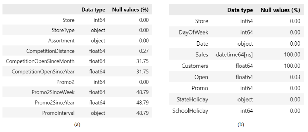
Figure 1. Missing values in store (a) and test (b) dataset
Different treatment will be given to each column with missing values. Every row in store dataset holds information regarding a specific store, hence row with missing values can’t be deleted regardless its high percentage. Thus, a mode will be imputed. By checking the value of Promo2 that corresponds to rows with missing value in Promo2SinceWeek, Promo2SinceYear, and PromoInterval, it can be observed that missing values in those three columns are caused by the store that did not participate in Promo2, thus the missing values here are logically correct. In order to give valid number in these columns, constant number 0 will be imputed. Meanwhile, the missing values in CompetitionDistance will be imputed with its maximum value.
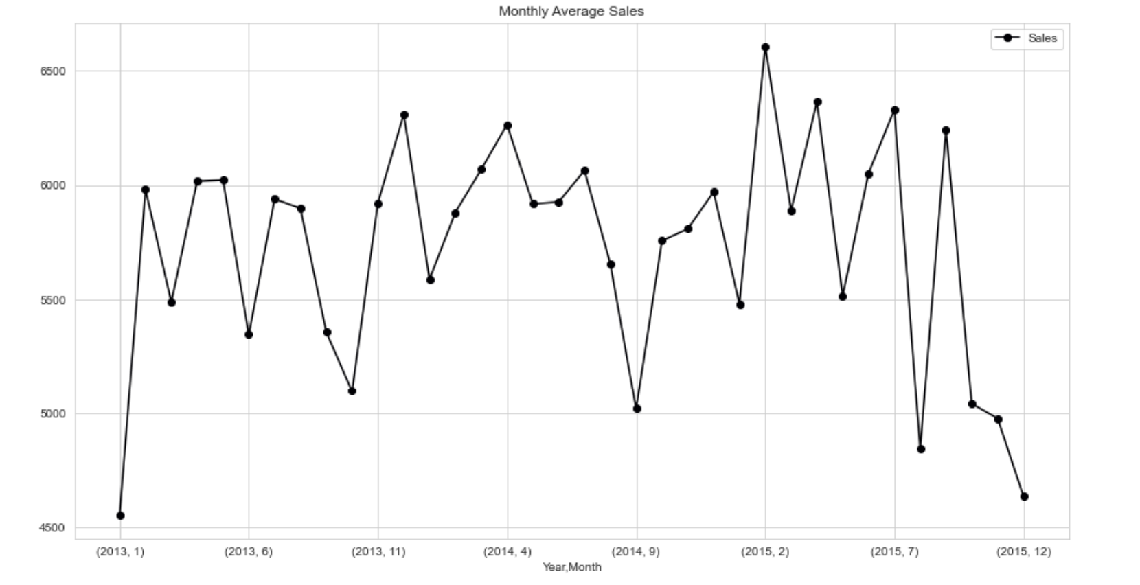
Figure 2. Monthly average of sales in Store 5 and 1114
From Figure 2, it can be observed that the sales reached its peak in the end of the year and smaller spike can be seen at the time of summer holiday.
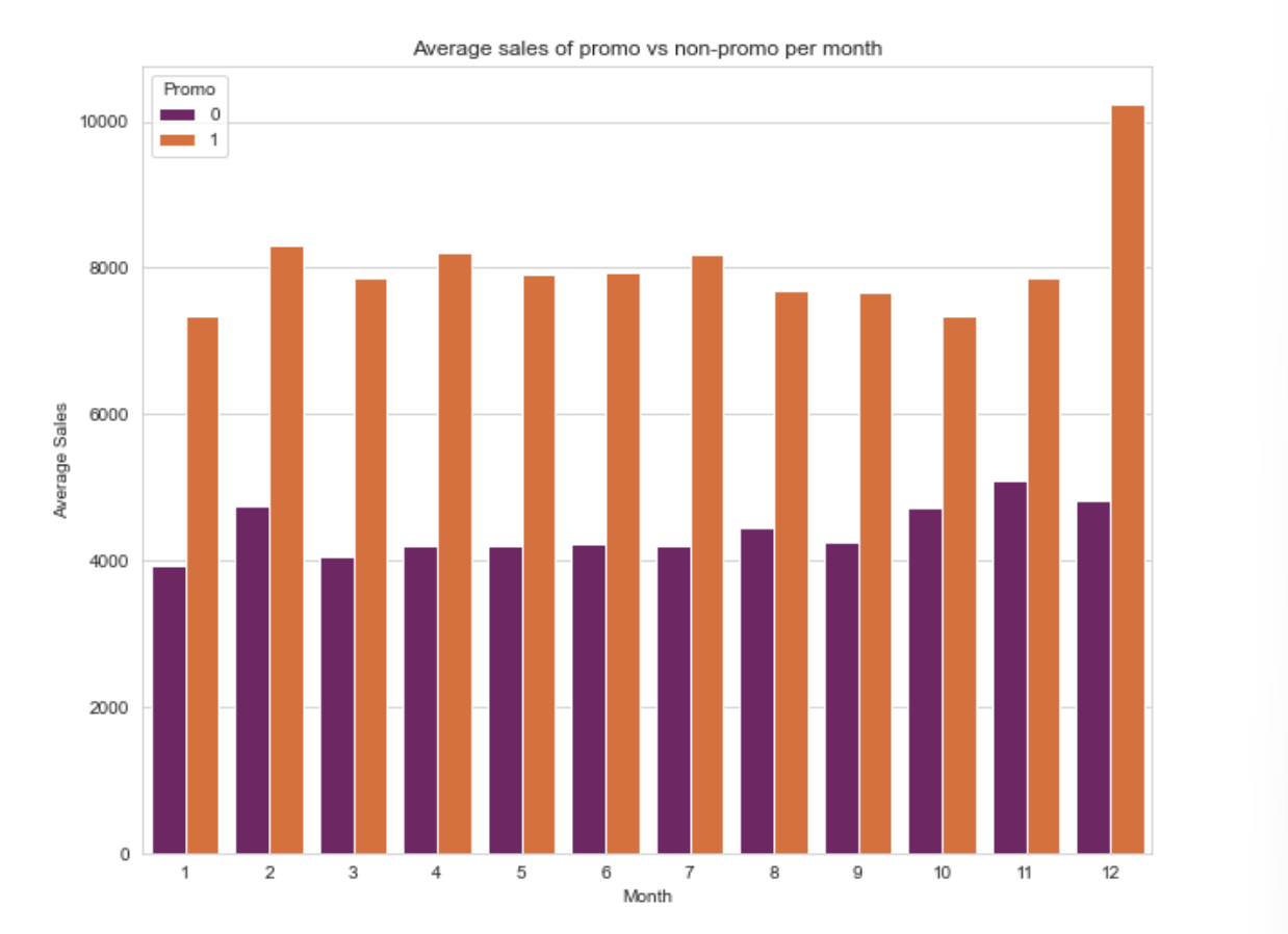
Figure 3. Average of sales with promo and non-promo in each month
Besides seasonality, sales data might be affected by promo that was offered by the store and days of the week as shown in Figure 3 and Figure 4 respectively. In Figure 3, days that offer promo to customers have higher average of sales than days with no promo, meanwhile Figure 4 shows that most of the stores were closed on Sunday so the average of sales on this day is the lowest compared to the other days. On the contrary, when only open store is considered then the sales on Monday and Sunday are the highest. Similar trend when average sales is higher when only opened store is considered but it is lower when both opened and closed store are considered also happen on State holiday as shown in Figure 5.
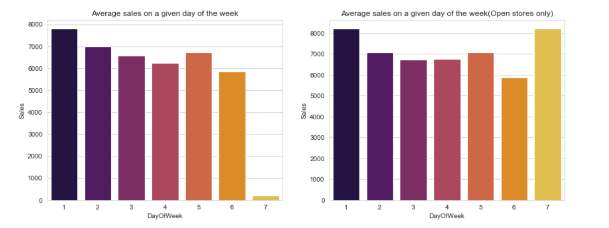
Figure 4. Average sales per day of the week
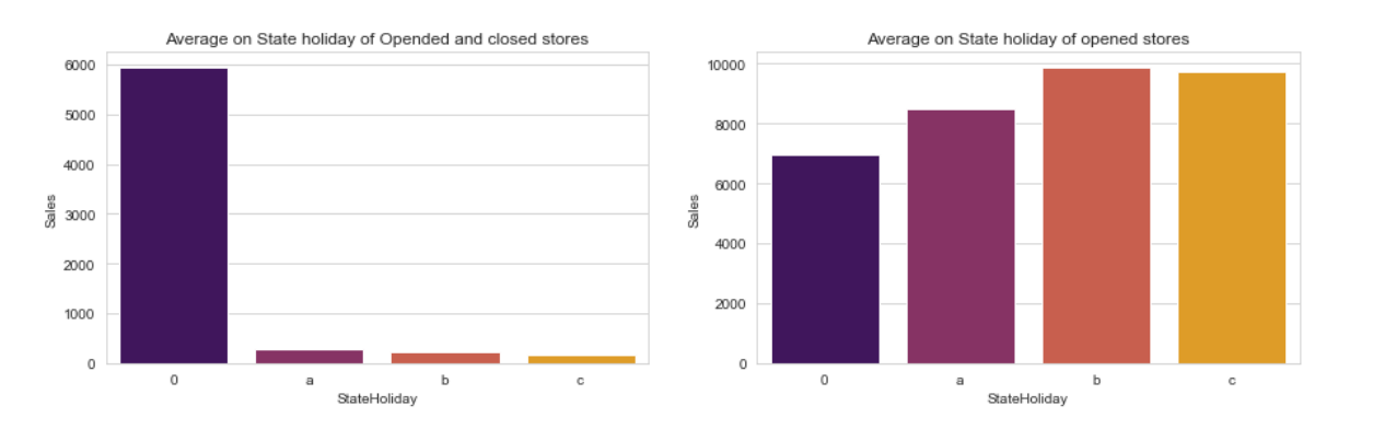
Figure 5. Average of sales on State holiday
Sales data might be affected by the presence of competitor. Figure 6 shows that the monthly average sales of a store decrease after the date its competition opened. The monthly average of Store 269 is more affected by competition than Store 5 and it’s caused by the difference on the distance between stores and competitor.
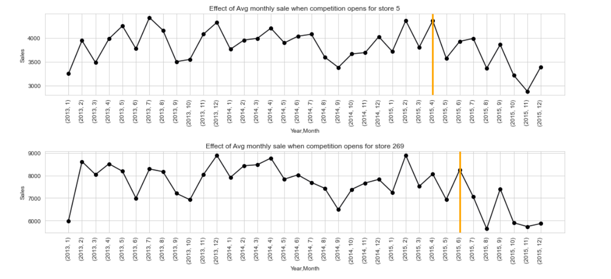
Figure 6. Average sales after competitor opened
Besides specific promo that was offered by store, a store can also join continuous and consecutive promotion that is coupon based, named Promo2. In Figure 7, the average daily sales in Store 500 after coupon was reactivated is shown.
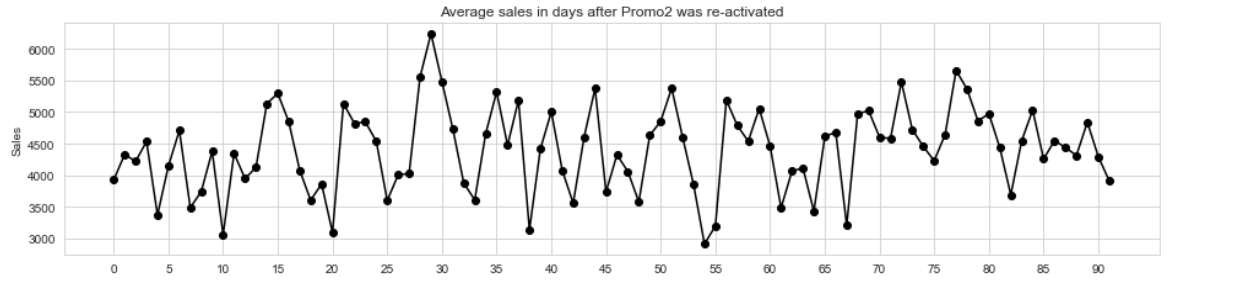
Figure 7. Average sales in days after Promo2 was re-activated in Store 500
At first, several features were made based on value in other column, such as:
Month,Day,WeekOfYearthat were extracted fromDateby using function in datetime. These variables help to explain the cyclic variation of the data.CompetitionOpenthat indicates the number of days since the competition was opened.PromoOpenthat indicates the number of days since the coupon of Promo2 was re-activated in an interval.Promo2is assumed to be re-activated on first day of the month inPromoInterval.IsPromoMonththat is a boolean where the value will be 1 if the month of aDateis in thePromoIntervalwhenPromo2coupon is being re-activated.Promo2gather information by comparingPromo2start date andDate(if the start date is later than theDate, 0 value is given or else 1).
Some features that have less than 0.01 correlation with Sales as shown in Figure 8 will be dropped. Besides that, the prediction model is made based on train data where sales data exist (sales > 0), thus any row with Open = 1, Customers = 0, and Sales = 0 will be dropped.
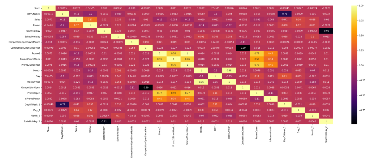
Figure 8. Correlation coefficient of predictor to target variable (Sales)
Before being used in training, the train and test dataset were linked or merged with store dataset on their common column Store. Training was done for each store, thus the result will be a prediction model for each store. When this is done, the value in some features such as CompetitionDistance, StoreType, and Assortment will not vary thus this feature will be dropped. Compared to the number of observation (n) for each store in train dataset, the number of features (p) is considered small thus feature reduction is not needed.
Assumptions
- The null values in three stores are assumed to be caused by both stores that located adjacent to each other, hence they are highly competitive.
- Schools remain closed on weekends and state holidays
- Store opening on holidays depends on each store.
Methodology
Linear Regression
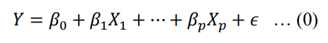
With multiple predictors, the linear regression model predicts the target variable by following below equation
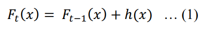
XGBoost By assuming that model parameters have been optimized, gradient boosted is shown to be the best learning method out of all decision trees-based algorithm [3]. Similar to random forest, it combines many decision trees to produce the final prediction. The term ‘boosted’ means that the model is build by adding weak learner (a decision tree) in each step to produce a strong learner. In general, gradient boosted in tth step try to find the new decision tree h(x) that correct the error or correct residual of the model in t-1th step and minimize the objective function (1).
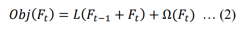
In XGboost, a new decision tree is added to minimize the object function (2), where L(Ft) is loss function and Ω(𝐹𝑡) refer to regularisation that is important to prevent over-fitting.
The final equation that will be used to determine each feature splits in a node in XGBoost is explained by the gain function in (3) that should be maximized.
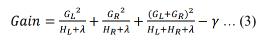
where
- L and R: to left and right nodes
- y: penalty
- lambda: L2 leaf weight penalty
XGBoost needs some parameters that should be selected. Determining the value of parameters that optimize above functions is not clear, thus it is done by assuming. Several parameters that are used are shown in Table 2, and complete list of parameters are explained in [4].
| Parameters | Explanation |
|---|---|
objective |
Learning objective function |
booster |
Booster to use |
eta |
Shrinkage term |
max_depth |
Maximum tree depth for base learners |
subsample |
Ratio subsample of the training set |
colsample_bytree |
Subsample ratio of columns when constructing each tree |
seed |
Used to generate folds |
The scoring method Root Mean Square Percent Error (RMSPE) is used to evaluate the forecasting accuracy
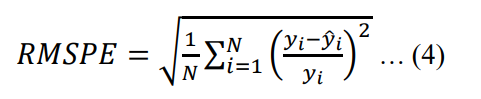
where N is the number of observed data, 𝑦𝑖 is the actual sales and 𝑦̂𝑖 is the predicted sales on ith observation.
In the merged dataset, there are some non-ordinal data such as Day, WeekOfDay, Month, and
StateHoliday. These features can cause problem even though in XGBoost from version 1.5 onwards can
handle this, thus some pre-processing step need to be done. Three types of method can be chosen to handle this case: one-hot encoding, ordinal encoding, and imposing order. For the Rossmann dataset, the third option is chosen because one-hot encoding can be slow for features with many distinct value [6], meanwhile ordinal encoding just assigns integer value to each category. By using imposing order, the mean of target variable for each category is used to replace non-ordinal data.
Lastly, while training the model we can specify the number of boosting iterations in num_boost_round.
Result and Analysis
The final predictor that are used are DayOfWeek, Promo, StateHoliday, SchoolHoliday, Promo2, PromoOpen, IsPromoMonth, Day, and Month. The linear regression models resulted in validation score of 0.49158 RMSPE. This value is higher that RMSPE that was obtained with XGBoost model which is 0.17047. After implementing different weighting in the sales prediction with XGBoost model, the validation score of 0.16909 RMSPE is obtained. There is variation on the RMSPE in each store, it’s due different characteristics or sales trend in each store so the chosen parameters might need to be adjusted.
Finally, the number of iterations can either being stopped when it reached the num_boost_round or once the eval-rmse increase again because the early_stopping_rounds is set to 1. Because of the restrictions in hardware capacity, the num_boost_round is set to 250 when training each model for 1,115 stores. In all training process, the iteration stopped after the 250th iteration. This means that with higher num_boost_round, a better RMSPE score might be obtained.
Conclusion and Recommendations
XGBoost model performs better than multiple linear regression, with cost of higher computation power and time. Lower RMSPE score from XGBoost model is obtained after applying weighting for each different store. By applying this method, the RMSPE score decrease from 0. 17047 to 0.16909. There are some methods that could be applied for future work, such as:
- Combine the original dataset with external data that helps in explaining the external factors influencing the store’s sales, such as weather data, German state, and google search trends [5].
- Choose machine with higher computational power might help in the training process with XGBoost
because if affect the number of
num_boost_roundthat could be set to make sure the lowest eval-rmse is obtained. - Cluster the store based on their pattern of sales data and build model for each store-cluster instead of a model for each store because building 1,115 model requires high computational power and time.
References
- Singh, T. (2015). Forecasting Rossmann Sales Figures Chris Jee (cjee).
- Lin, S., Yu, E., Guo, X. (2015). Forecasting Rossmann Store Leading 6-month Sales CS 229 Fall 2015
- Hastie, T., Tibshirani, R., & Friedman, J. (2009). The Elements of Statistical Learning: Data Mining, Inference, and Prediction, Second Edition. Springer Publishing.
- Python API Reference—xgboost 2.0.0-dev documentation. (n.d.). https://xgboost.readthedocs.io/en/latest/python/python_api.html
- Rossmann Store Sales | Kaggle. (n.d.). https://www.kaggle.com/competitions/rossmann-store-sales
- Korolev, M.V., & Ruehh, K. (2015). Gradient Boosted Trees to Predict Store Sale