A project to predict whether a woman has diabetes based on their health records.
Author: Ninda Khoirunnisa. This is coursework for Statistic and Machine Learning I: Statistical Foundations Course in MSc Data Science Program, University of Manchester, 2022.
Dataset Description
This term dataset that is used here refer to the data that was collected from Pima Indian population by National Institute of Diabetes and Digestive and Kidney Disease [1]. The population is 750 women, and in each recorded data there are 8 features (independent variable) and 1 outcome (dependent variable).
Eight features that are used as diagnostic measure in this dataset are explained in Table 1 below
| Variables | Description |
|---|---|
| Prenancies | Number of times a women get pregnant |
| Glucose | Plasma glucose concentration at 2 hours in Oral Glucose Tolerance Test (GTT) |
| Blood pressure | Diastolic blood pressure (mm Hg) |
| Skin thickness | Triceps skin fold thickness (mm) |
| BMI | Body mass index (weight in kg/(height in m)^2) |
| Diabetes pedigree | A synthesis of the diabetes mellitus history based on the expected genetic influence of affected and unaffected relatives on the subject’s eventual diabetes risk (Smith et al., 1988). |
| Age | Age (years) |
One of data quality measure is the completeness of data, that is reflected by how many missing values. In this dataset, there are no explicit null values as shown in Figure 1 below. But by observing the minimum value from the summary of the dataset as shown in Figure 2, there are records with 0 value. These records will be assumed as having null values because it is logically incorrect.

Figure 1. Data type and missing value of each feature
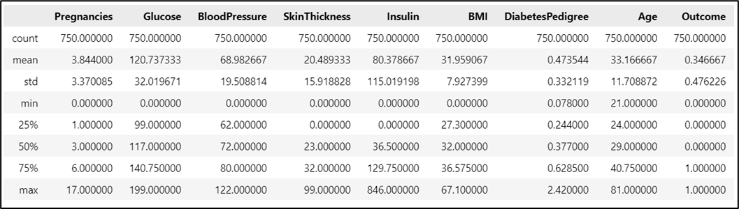
Figure 2. Summary of numeric values in the dataset
Exploratory Data Analysis
After replacing the 0 value with null, the number of non-missing values is recalculated and the result is shown in Figure 3.
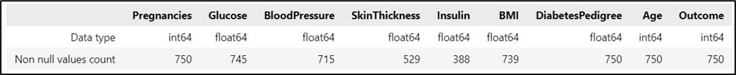
Figure 3. Recalculation result of missing values
Bar and pie plot are used to visualize the ratio of data that are classified as 1 and 0 as shown in Figure 4. It shows that the dataset is unbalanced.
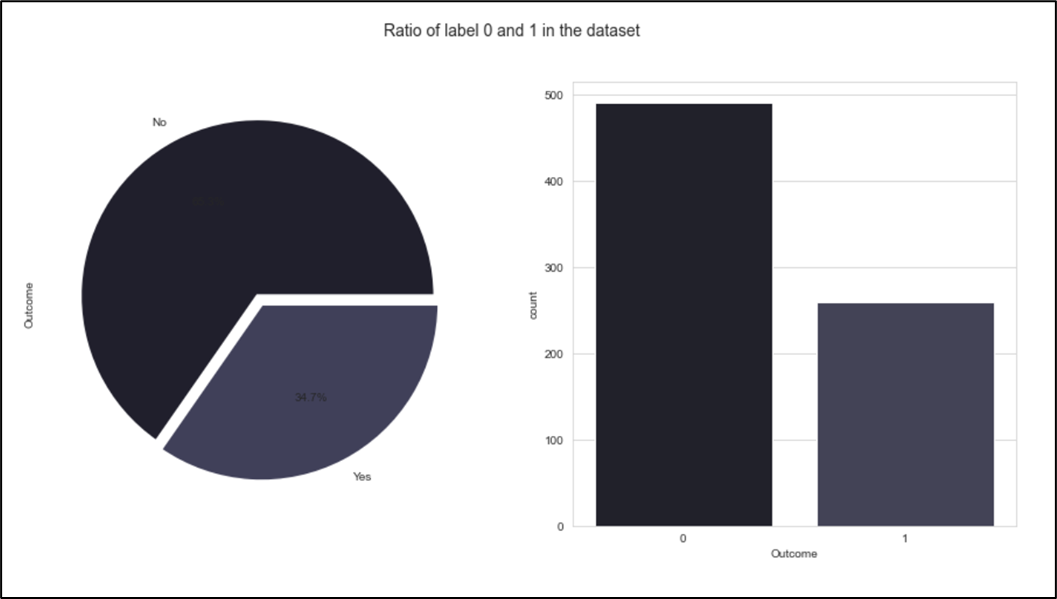
Figure 3. Distribution of the label Income
In this dataset, the correlation of each feature is visualized as heatmap in Figure 5 below.
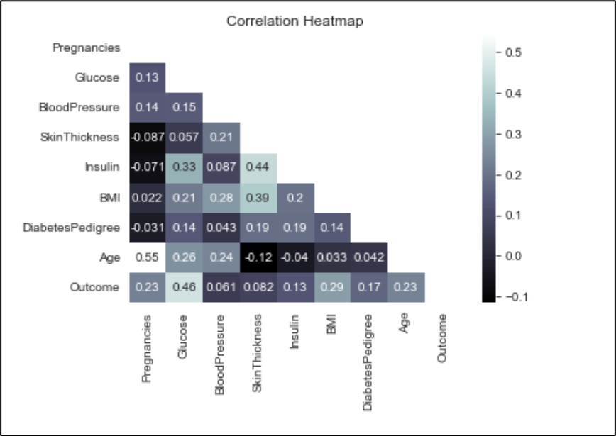
Figure 5. Correlation between features
Correlation between features in PimaDiabetes dataset range from 0 to 1. All features have positive correlation with Outcome, and feature Glucose has the highest positive correlation meanwhile BloodPressure has the lowest correlation with Outcome.
Before visualizing the distribution of each feature, to ease the comparation process the data will be standardized by following this equation
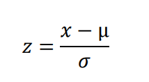
The visualisation of the distribution of the standardized PimaDiabetes is shown in Figure 6.
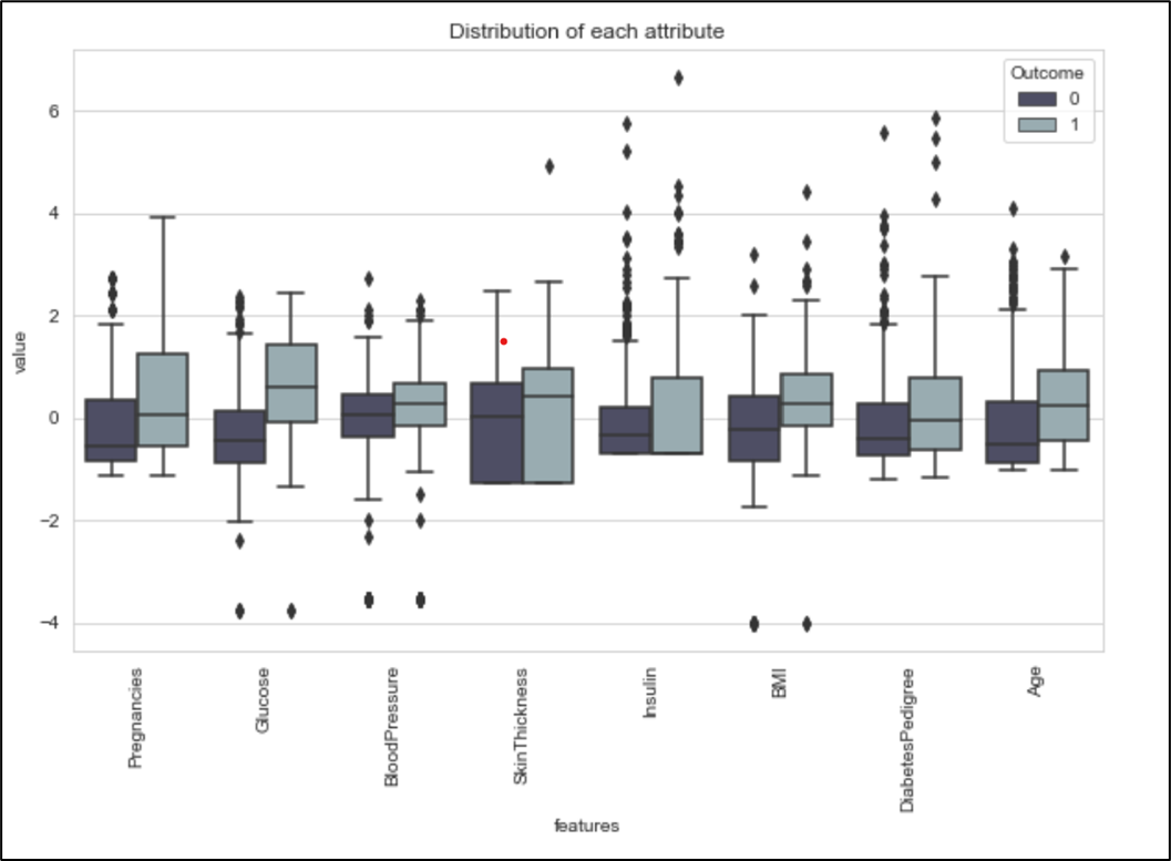
Figure 6. Boxplot of PimaDiabetes
What can be concluded from the boxplot above are:
- The distribution in
Age,DiabetesPedigree,Insulin,SkinThickness, andPregnanciesare skewed to the right. - The distribution in
Glucose,BloodPressure, andBMIare symmetric and uniform. - Zero values in
Glucose,BloodPressure, andBMIare considered as outliers, meanwhile inSkinThicknessandInsulinthose are not because it took up a big part of the data.
It is known that there are outliers in every feature. Also, the trend shows that the median of features whose Outcome is 1 is higher than the data whose Outcome is 0. To illustrate the correlation between two features, the pair plot is used as shown in Figure 7. By looking at this visualisation, the Glucose is assumed to be the best estimator because the scatter plots between Glucose and other features are the most clearly separated.
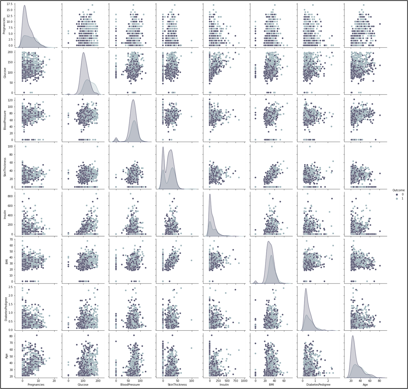
Figure 7. Pairplot
Regression Model with Single Predictor
A column ThreeOrMoreKids is filled with boolean value that represents whether a sample ever got pregnant thrice or more, or not. The comparation of data with True and False value in this column is shown in Figure 8.
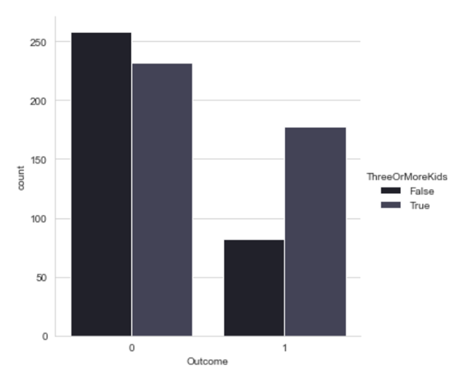
Figure 8. Bar plot of ThreeOrMoreKids column’s value against its count
There are more non-diagnosed women who have less than three kids but there are more diabetes diagnosed women who have three or more kids. It indicates the positive correlation between ThreeOrMoreKids and Outcome.
According to Alan et.al., regression model for binary responses describes the population proportions. The intercept and coefficient from LogisticRegression, calculated by scikit-learn, are shown in Figure 9 below.
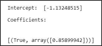
Figure 9. Intercept and coefficient from LogisticRegression
Since the estimate 0.859 of β is positive and 1 represent True (have three or more kids), the estimated probability of a women to be diagnosed positive increases for women who have three or more kids.Since 1 in ThreeOrMoreKids indicate having three or more kids, the positive sign in the coefficient means that the estimated odds of diagnosed positive of diabetes are higher.
The alternative equation for logistic regression expresses the estimated probability of success directly by this following equation.
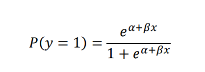
Since the Outcome only have two categories, a single dummy variable can represent each. Thus, by substituting the intercept and coefficient in Figure 3.6, the estimated probability of P(Outcome = 1 | ThreeOrMoreKids = False) = 0.427065, and P(Outcome = 0 | ThreeOrMoreKids = False) = 1 – 0.427065 = 0.572935. Meanwhile, the estimated probability of P(Outcome = 1 | ThreeOrMoreKids = True) is 0.432051553 and P(Outcome = 0 | ThreeOrMoreKids = True) = 1 – 0. 432051553= 0.56794845.
Regression Model
Data Preparation
- Features with many missing values such as
SkinThicknessandInsulinhas high correlation withBMIandGlucoserespectively, so to prevent high number of reduced rows if null values are dropped, bothSkinThicknessandInsulinwill be removed. - Missing value in other features will be imputed with median of each feature according to its label, since the distribution of these features are skewed.
- Outliers will be deleted because it contributes to the skewness of the data.
Fitting the model
LogisticRegression() from scikit-learn will provide intercept and coefficient for each feature as shown in Figure 4.1. These values can be used to calculate the estimated probability of women to be diagnosed positive given the continuous value in Pregnancies, Glucose, BloodPressure, BMI, DiabetesPedigree, and Age.
Before fitting the model, the data will be splitted into training and testing data with StratifiedShuffleSplit() to maintain the same proportion of ‘Glucose’ value because this feature has the highest correlation with Outcome. It is also done to test the performance of the model.
The features used as predictor affect the performance of the regressor model. Figure 10 and 11 shows the difference in accuracy when the number of features used is modified. The importance of each feature is defined by SelectKBest and chi2 in feature_selection from scikit learn. It uses chi-square for feature selection purpose.
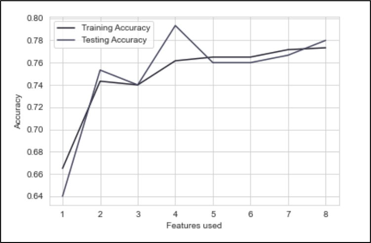
Figure 10. Number of features vs accuracy before imputing median to missing values and deleting SkinThickness & Insulin
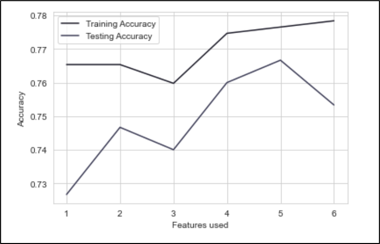
Figure 11. Number of features vs accuracy after imputing median to missing values
After the pre-processing is done, the intercept and coefficients for each feature is shown in Figure 12.
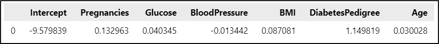
Figure 12. Intercept and coefficient of logistic regression
All features except BloodPressure have positive sign. Since the data is continuous, the estimated odds of women to be diagnosed positive of diabetes will increase as the data value becomes higher. On the other hand, BloodPressure has negative sign thus it will decrease the estimated probability of a women to be diagnosed positive when its BloodPressure value becomes higher.
According to Alan et. al., the farther a 𝜷𝒊 falls from 0, the stronger its effect on predictor xi and the odd ratios will fall farther from 1. Thus, for the coefficient in Figure 12, the predictor that has strong effect on xi are DiabetesPedigree. But this can also be affected of the different scale of each data.
On the first row data in ToPredict.csv, the estimated probability of this women to be tested positive is 0.558. Given the continuous value in 6 selected features, the estimated probability of this woman to be labelled 1 is higher than 1 – 0.558 = 0.442, and the odds equals 0.558/0.442 = 1.26, meaning that a positive diabetes test result is 1.26 times as likely as a non-diabetes. Predicted labels for all data in ToPredict.csv are shown in Figure 13.
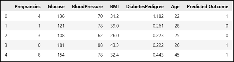
Figure 13. Predicted outcome of ToPredict.csv
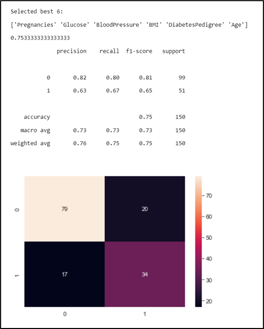
Figure 14. Model performance
Model Comparison
By observing the Figure 11, 5 features (Pregnancies, Glucose, BloodPressure, BMI, and Age) will be used as predictor in the second model because it gives the best accuracy in the testing data. The significance of these features is measured by using chi2 from feature_selection in scikit learn. The result of the calculation is shown in Figure 15 below.
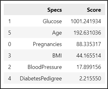
Figure 15. Feature significance
The intercept, coefficients, and predicted value of this model is shown in Figure 16 and 17 below.
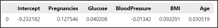
Figure 16. Intercept and coefficient of 5 features
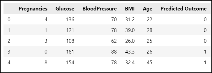
Figure 17. Predicted Outcome of ToPredict.csv
The performance of this model can be measured with confusion_matrix that shows how well the model classify the data.
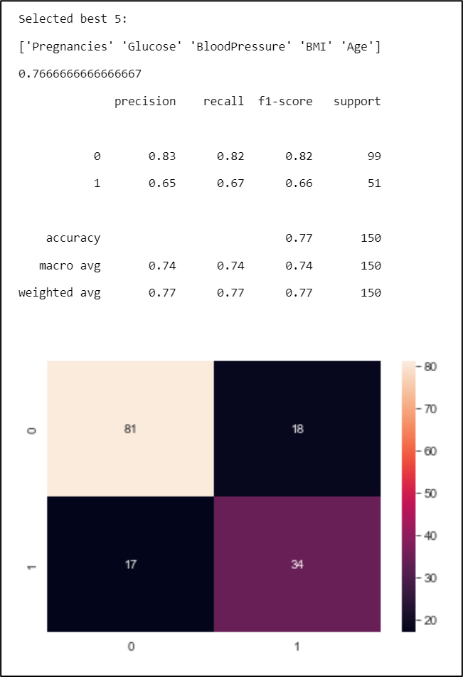
Figure 18. Model performance
Due to the imputation on the missing value, the distribution of data is slightly changed. Thus, the model with 6 features as predictor will be used to predict the status of each woman whether they are diagnosed with diabetes or non-diagnosed.
References
- Jack W. Smith, J.E. Everhart, W.C. Dickson, W.C. Knowler, & R.S. Johannes. (1988). Using the ADAP Learning Algorithm to Forecast the Onset of Diabetes Mellitus. Annual Symposium on Computer Application in Medical Care, 261–265.
- Agresti, A. (2018). Statistical Methods for the Social Sciences, Global Edition (5th edition). Pearson Education Limited.
- sklearn.feature_selection.chi2. (n.d.). Scikit-Learn. https://scikit-learn.org/stable/modules/generated/sklearn.feature_selection.chi2.html
- Step by Step Diabetes Classification-KNN-detailed. (2020, October 31). Kaggle. https://www.kaggle.com/code/shrutimechlearn/step-by-step-diabetes-classification-knn-detailed
- Multivariate Statistical Analysis on Diabetes. (2020, August 10). Kaggle. https://www.kaggle.com/code/ravichaubey1506/multivariate-statistical-analysis-on-diabetes
- Machine Learning & Predictive Modeling Analytics. (2020, April 16). Kaggle. https://www.kaggle.com/code/ravichaubey1506/machine-learning-predictive-modeling-analytics?scriptVersionId=3211447