This project aimed to segment customers of an online retail store based on their similarity in behaviour and to find patterns in the data.
Author: Ninda Khoirunnisa. This is coursework for Data Engineering Course in MSc Data Science Program, University of Manchester, 2022.
Customer Segmentation
EDA
This Online Retail II data set (from here) contains all the transactions occurring for a UK-based and registered, non-store online retail between 01/12/2009 and 09/12/2011.The company mainly sells unique all-occasion gift-ware. Many customers of the company are wholesalers.
We’re going to investigate whether there are groups of customers, how they are similar, and what they may represent.
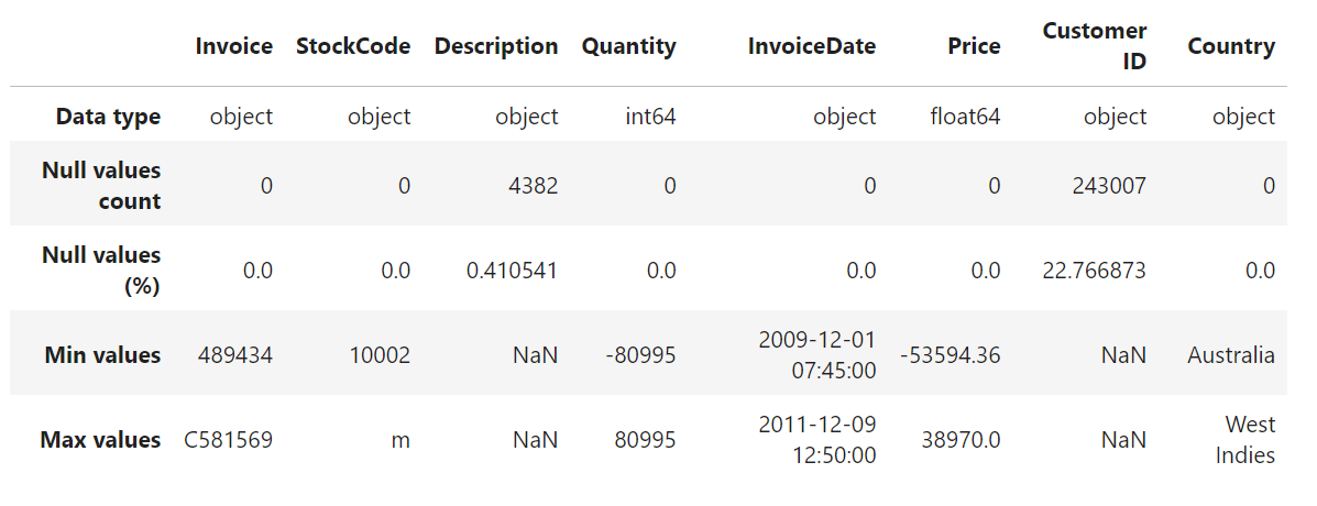
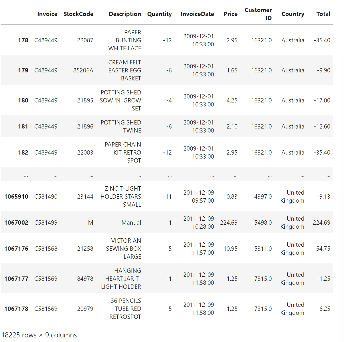
Figure 1. About the dataset
The colum InvoiceDate has datatype = object, thus the data type should be changed to datetime. Besides that, the row with null value in column Customer ID will be dropped because this data is considered important and there is no way to impute the data. A new column Total is added to show the amount of payment made for each product in an invoice. Figure 2 shows the result after manipulating the data.
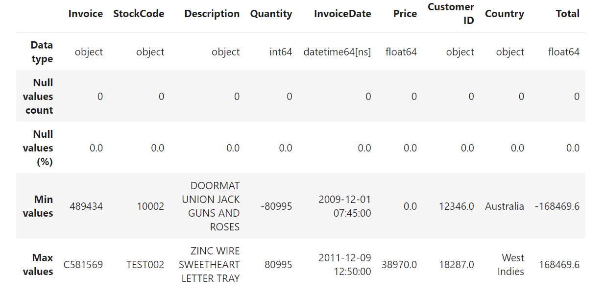
Figure 1. Description of the dataset after data manipulation
The code below is used to count the duplicated row in this dataset with function duplicated(). Any duplicated row will be deleted after that.
print('Number of duplicate: {}'.format(retail.duplicated().sum()))
retail.drop_duplicates(inplace=True)
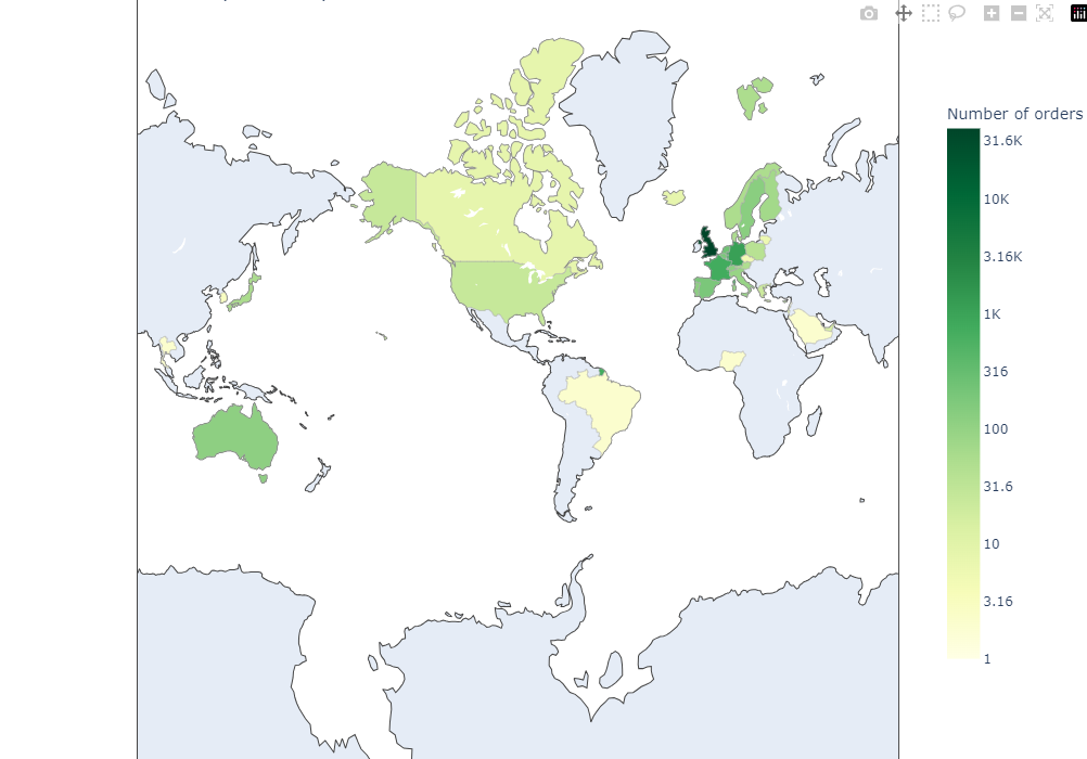
Total order per country
Line of codes below are used to create more readable text on the map’s legend, for example if a number is 10000 it will be writter ‘10K’ on the map. To visualize data on the map (choropleth), the retail dataset will be grouped by Customer ID, Invoice, and Country. The highes total order/invoice in a country, the darker its colour will be.
Because the range of number of invoice in each country is high, log function with base = 10 is used. From the visualization, most invoice is made by people in Europe continent with UK as the country with most invoice/orders.
def human_format(num):
    num = float('{:.3g}'.format(num))
    magnitude = 0
    while abs(num) >= 1000:
        magnitude += 1
        num /= 1000.0
    return '{}{}'.format('{:f}'.format(num).rstrip('0').rstrip('.'), ['', 'K', 'M', 'B', 'T'][magnitude])
temp = retail[['Customer ID', 'Invoice', 'Country']].groupby(['Customer ID', 'Invoice', 'Country']).count()
temp = temp.reset_index(drop = False)
countries = temp['Country'].value_counts()
tickvals = [0, 0.5, 1, 1.5, 2, 2.5, 3, 3.5, 4, 4.5]
data = dict(type='choropleth',
            locations = countries.index,
            locationmode = 'country names', z = np.log10(countries),
            customdata=countries,hovertemplate=
            "Number of orders: %{customdata}",
            colorscale=('YlGn_r'),
            colorbar=dict(len=0.75,
                  title='#Cases',
                  x=0.9,
                  tickvals = [0, 0.5, 1, 1.5, 2, 2.5, 3, 3.5, 4, 4.5],
                  ticktext = list(map(lambda x: human_format(10**x), tickvals))),
            reversescale = True,
            marker_line_color='darkgray',
            marker_line_width=0.5,
            colorbar_title='Number of orders')
layout = dict(title='Number of orders per country',
geo = dict(showframe = True, projection={'type':'mercator'}), width=1000, height=700)
choromap = go.Figure(data = [data], layout = layout)
choromap.update_layout(margin={"r":0,"t":0,"l":0,"b":0})
iplot(choromap, validate=False)
Cleaning the data
Dealing with the cancelled invoice
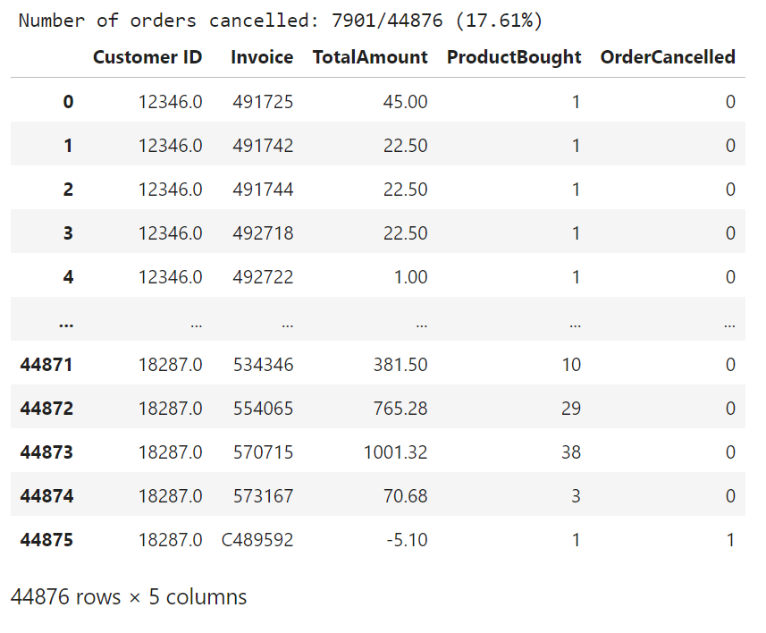
To further gaining insight from this dataset, some cleaning must be done because as seen below there are orders with negative TotalAmount. By filtering the data to show only row with negative TotalAmount value, Invoice with prefix ‘C’ will be obtained. Thus, Invoice with this prefix will be assumed as cancelled order.
From this dataset, 7901 order are found cancelled.
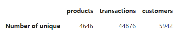
pd.DataFrame([{'products': retail['StockCode'].nunique(),
               'transactions': retail['Invoice'].nunique(),
               'customers': retail['Customer ID'].nunique(),
              }], columns = ['products', 'transactions', 'customers'], index = ['Number of unique'])
r = retail.groupby(by=['Customer ID','Invoice'], as_index=False)['Total'].agg(['sum','count']).reset_index().rename(columns={'sum': 'TotalAmount', 'count': 'ProductBought'})
r.sort_values('Customer ID')[:15]
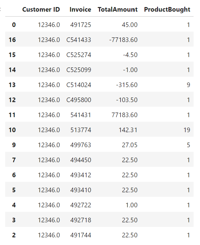
r['OrderCancelled'] = r['Invoice'].apply(lambda x:int('C' in x))
n1 = r['OrderCancelled'].sum()
n2 = r.shape[0]
print('Number of orders cancelled: {}/{} ({:.2f}%) '.format(n1, n2, n1/n2*100))
display(r)
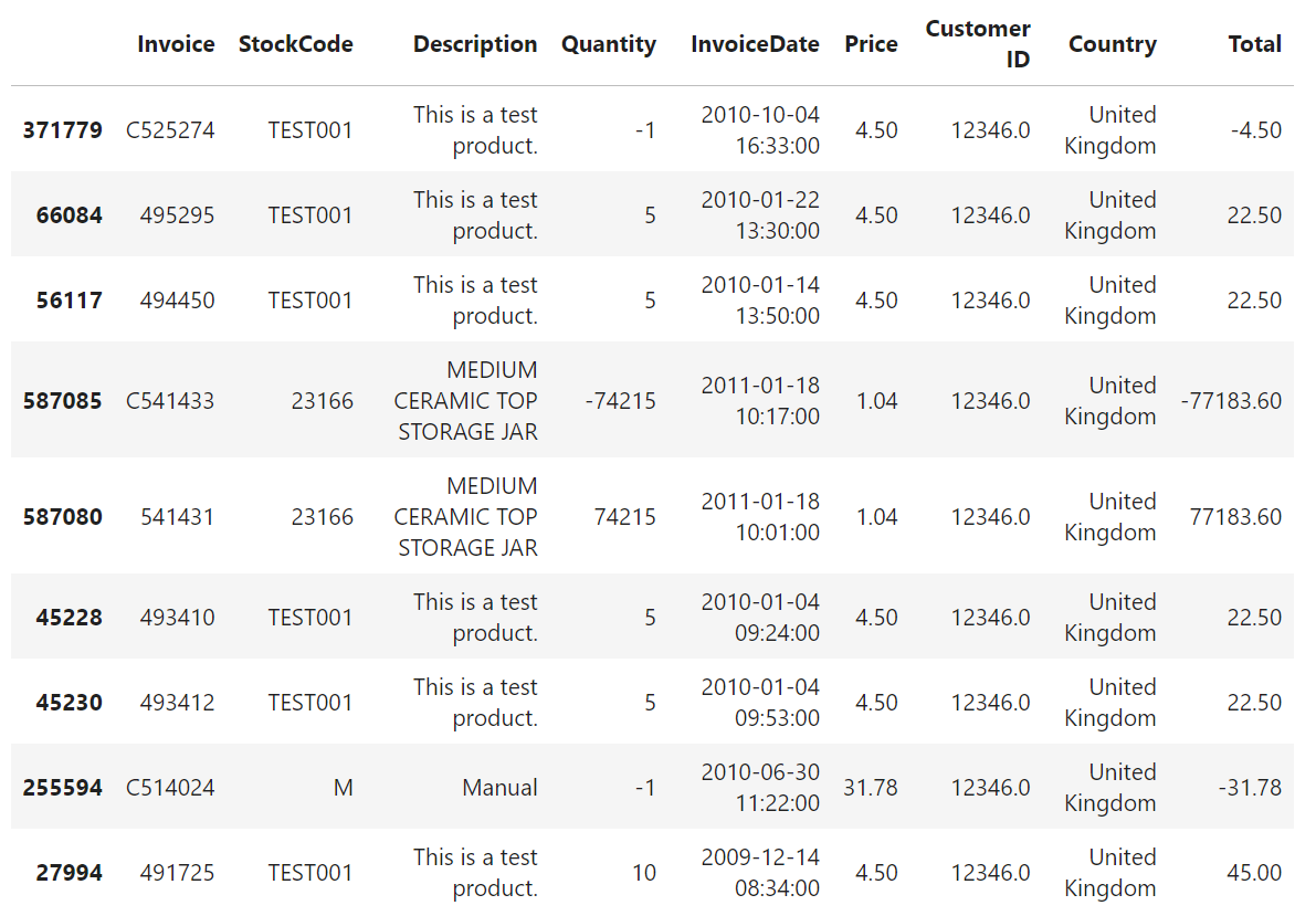
By checking the StockCode that contain alphabet, it can be known that there are several testing data. This kind of data will not be considered as order data by real user, so in the next cell this kind of data will be removed from new dataframe named df_check.
display(retail.sort_values('Customer ID')[16:25])
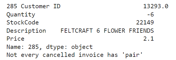
The code below is used to check wether a cancelled invoice has pair with the same value of Customer ID, Quantity, and Description. Because not every cancelled order/invoice has pair, a new dataframe named df_dirty will be made to accommodate only data whose Quantity is less than 0 and it is not a discount.
In order to check and iterate over all rows to get a pair of data with positive and negative TotalAmount with the same Customer ID, Quantity, and Description, a new dataframe named df_pos is made.
df_check = retail[(retail['Quantity'] < 0) & (~retail['Description'].isin(list_special_codes))][
                                 ['Customer ID','Quantity','StockCode',
                                  'Description','Price']]

for index, col in  df_check.iterrows():
    if retail[(retail['Customer ID'] == col[0]) & (retail['Quantity'] == -col[1])
                & (retail['Description'] == col[3])].shape[0] == 0:
        print(index, df_check.loc[index])
        print("Not every cancelled invoice has 'pair'")
        break
df_dirty = retail.copy()
df_dirty = df_dirty[(df_dirty['Quantity'] < 0) & (df_dirty['Description'] != 'Discount')]
df_dirty
retail['QuantityCancelled'] = 0

remove = []
remove_1 = []
suspicious = []

for index, col in  df_dirty.iterrows():
    if (col['Quantity'] > 0) or col['Description'] == 'Discount': continue
    df_test = df_pos[(df_pos['Customer ID'] == col['Customer ID']) &
                         (df_pos['StockCode']  == col['StockCode']) &
                         (df_pos['InvoiceDate'] < col['InvoiceDate']) &
                         (df_pos['Quantity'] > 0)].copy()

    if (df_test.shape[0] == 0):
        suspicious.append(index)

    elif (df_test.shape[0] == 1):
        index_order = df_test.index[0]
        retail.loc[index_order, 'QuantityCancelled'] = -col['Quantity']
        remove_1.append(index)
        #positive_1.append(index_order)

    elif (df_test.shape[0] > 1):
        df_test.sort_index(axis=0 ,ascending=False, inplace = True)
        for ind, val in df_test.iterrows():
            if val['Quantity'] < -col['Quantity']: continue
            retail.loc[ind, 'QuantityCancelled'] = -col['Quantity']
            remove.append(index)
            #positive.append(ind)
            break
After iteraning over all rows, this rules will be followed:
- If invoice with negative value has no pair, this rows will be dropped
- If invoice with negative value has one pair, its negative quantity will be added as new column
QuantityCancelledon its positive pair rows and the negative invoice will be dropped. - If invoice with negative value has more than one pair, its negative quantity will be added to
QuantityCancelledof one of its positive pair rows and the negative invoice will be dropped.
retail.drop(remove, axis=0, inplace=True)
retail.drop(suspicious, axis = 0, inplace = True)
retail.drop(remove_1, axis = 0, inplace = True)
retail.shape
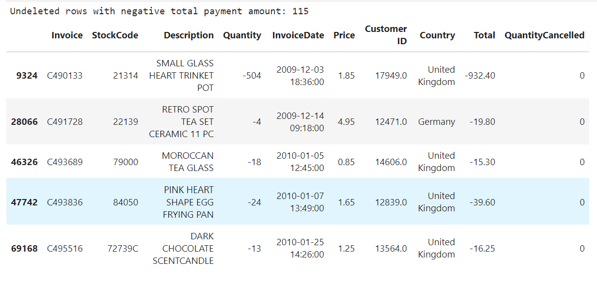
remaining_entries = retail[(retail['Quantity'] < 0) & (retail['StockCode'] != 'D')]
print("Undeleted rows with negative total payment amount: {}".format(remaining_entries.shape[0]))
remaining_entries[:5]
Dealing with one unique product with more than one description
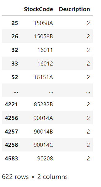
The number of unique value in StockCode and Description because there are 622 products that have more than one descriprions. The lines of code below are used to assign the min value of each Description to every Description column with the same StockCode value.
transaction_types = retail[retail['StockCode'].str.contains('^[a-zA-Z]+', regex=True)]['StockCode'].unique()
df_clean = retail.copy()
df_clean = df_clean[~df_clean['StockCode'].isin(transaction_types)]

df_desc = df_clean['Description'].str.lower().unique()
print("Number of unique description: {}".format(len(df_desc)))
prod = df_clean['StockCode'].unique()
print("Number of product: {}".format(len(prod)))

dff = df_clean.groupby(by=['StockCode'], as_index=False)['Description'].nunique()
dff.to_csv('prod_desc.csv')
dff[dff['Description'] >1]
dfs = df_clean.groupby(by=['StockCode', 'Description'], as_index=False)['StockCode', 'Description'].mean()
prod_desc = dfs.groupby(by=['StockCode'], as_index=False).min()
prod_desc

key_list = list(df_clean['StockCode'])
dict_lookup = dict(zip(prod_desc['StockCode'], prod_desc['Description']))

df_clean['Description'] = [dict_lookup[item] for item in key_list]
df_clean
Group of order/invoice based on each total payment
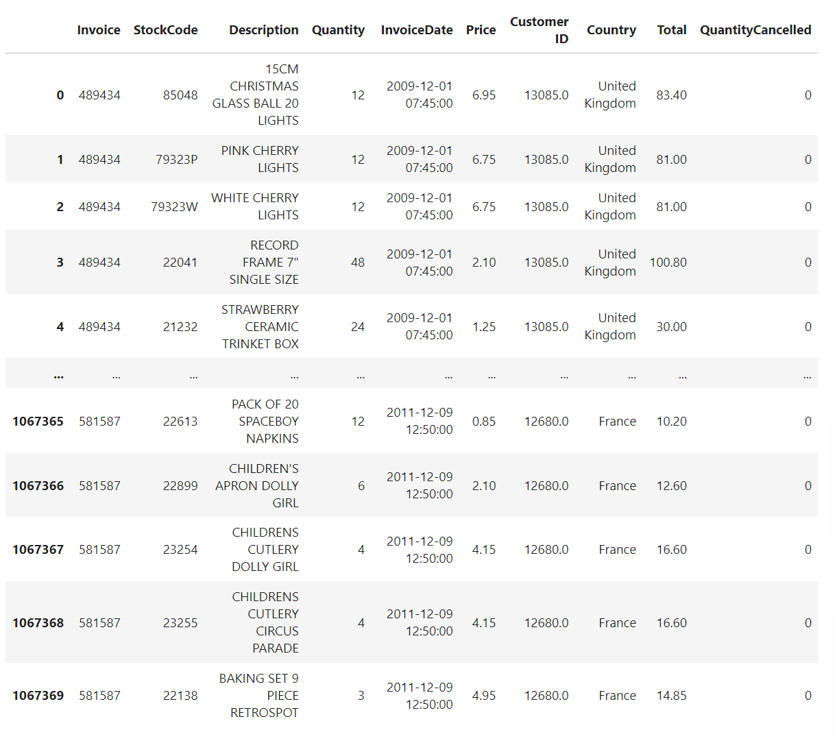
df_clean['Payment amount'] = df_clean['Total'] - (df_clean['Price'] * df_clean['QuantityCancelled'])
df_clean.sort_values('Customer ID')[:5]
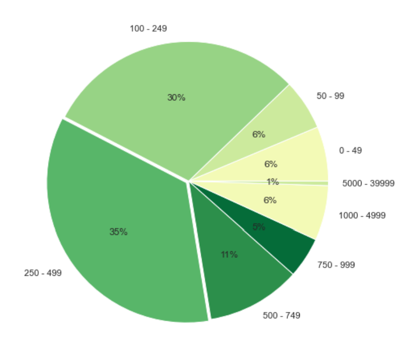
Line of codes below are used to group the df_clean dataframe by Customer ID, Invoice and InvoiceDate and show the total payment and total bought products in each invoice. This distribution of total amount from all invoices are then visualized in a pie chart.
r = df_clean.groupby(by=['Customer ID','Invoice', 'InvoiceDate'], as_index=False)['Payment amount'].agg(['sum','count']).reset_index().rename(columns={'sum': 'TotalAmount', 'count': 'ProductBought'})
s = df_clean.groupby(by=['Customer ID','Invoice'], as_index=False)['InvoiceDate'].max()
r['InvoiceDate'] = s['InvoiceDate']
r = r[r['TotalAmount'] > 0]
r.sort_values('TotalAmount')

r = r[r['TotalAmount'] > 0]
price_range = [0, 50, 100, 250, 500, 750, 1000, 5000, 40000]
count_price = []
for i, price in enumerate(price_range):
    if i == 0: continue
    xi = r[(r['TotalAmount'] < price) &
                       (r['TotalAmount'] > price_range[i-1])]['TotalAmount'].count()
    count_price.append(xi)
sns.set_style("whitegrid")
labels = [ '{} - {}'.format(price_range[i-1], j-1) for i,j in enumerate(price_range) if i != 0]
fig, ax = plt.subplots(figsize=(15, 8))
explode = [0, 0, 0, 0.02, 0,0,0, 0]

#create pie chart
plt.pie(count_price, labels = labels, colors = sns.color_palette('YlGn'), autopct='%.0f%%', explode=explode)
plt.figsize=(10,8)
plt.show()
Classify product into category
Each StockCode has description and from this column, product category can be generated. Before a clustering is conducted, the text data in column Description need to be preprocessed in stemming, tokenizing, deleting stopword, and checking the noun.
For the stemmer, porter stemmer will be used because according to [5], PorterStemmer is known for its simplicity and speed. Besides that, it is commonly used in information retrieval environments for fast recall and fetching of search engines.
Before stemming is done, each string in Description column will be lowered because of python’s case sensitivity. After that, each string will be tokenized by word_tokenize from nltk. Besides that, english stopword will also be removed. After this, only noun will be stemmed with PosterStemmer.
from nltk.corpus import stopwords
stopword = stopwords.words("English")

#from nltk.stem.lancaster import LancasterStemmer
from nltk.stem import PorterStemmer

is_noun = lambda pos: pos[:2] == 'NN'

def word_processing(df, c='Description'):
    stemmer = PorterStemmer()
    keyword_roots  = dict()
    keyword_select = dict()
    category_keys   = []
    count_keywords  = dict()
    icount = 0
    for i in df[c]:
        lowerc = i.lower()
        word_tokenized = nltk.word_tokenize(lowerc)
        sw = stopwords.words('english')
        sw_removed = [word for word in word_tokenized if not word in sw]
        nouns = [word for (word, pos) in nltk.pos_tag(sw_removed) if is_noun(pos)]

        for j in nouns:
            stemmed = stemmer.stem(j)
            if stemmed in keyword_roots:
                keyword_roots[stemmed].add(j)
                count_keywords[stemmed] += 1
            else:
                keyword_roots[stemmed] = {j}
                count_keywords[stemmed] = 1

    for s in keyword_roots.keys():
        if len(keyword_roots[s]) > 1:
            min_length = 1000
            for k in keyword_roots[s]:
                if len(k) < min_length:
                    clef = k ; min_length = len(k)
            category_keys.append(clef)
            keyword_select[s] = clef
        else:
            category_keys.append(list(keyword_roots[s])[0])
            keyword_select[s] = list(keyword_roots[s])[0]

    print("Number of keywords in variable '{}' : {}".format(c, len(keyword_roots)))
    return category_keys, keyword_roots, keyword_select, count_keywords

pd.DataFrame(df_clean['Description'].unique()).rename(columns = {0: 'Description'})

df_desc = df_clean['Description'].str.lower().unique()
df_descc = df_clean.groupby(by=['StockCode'], as_index=False)['Description'].min()
df_descc['Desc'] = df_descc['Description']
df_descc['Description'] = df_descc['Description'].str.lower()
df_descc

category_keys, keyword_roots, keyword_select, count_keywords = word_processing(pd.DataFrame(df_clean['Description'].unique()).rename(columns = {0: 'Description'}))

counts = pd.DataFrame.from_dict(count_keywords, orient='index').reset_index().rename(columns={'index': 'Words', 0: 'Frequency'}).sort_values('Frequency', ascending=False)
df_count = counts.iloc[0:100]
dfc = df_count.iloc[0:10]
fig, ax = plt.subplots(figsize=(7, 7))
dfc.sort_values(by='Frequency').plot.barh(x='Words',
                      y='Frequency',
                      ax=ax,
                      color='green')
plt.xticks(fontsize = 15)
plt.yticks(fontsize = 13)
plt.yticks()
plt.title('Number of occurrence of each words')
plt.show()
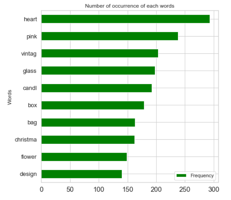
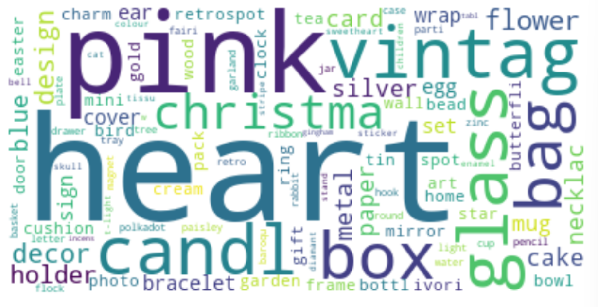
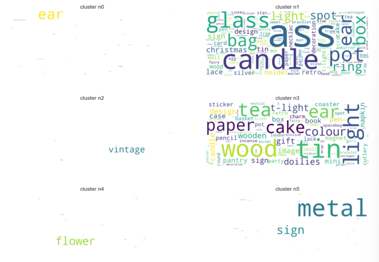
The bar plot and wordcloud above are used to visualize the most frequent words. Because there are thousands word from all Description, only word with or more than three letters and word whose frequency is more than or equal to 15 will be considered.
list_products = []
dict_products = {}
for k, v in count_keywords.items():
    word = keyword_select[k]
    if word in ['pink', 'blue', 'white', 'tag', 'green', 'orange']: continue
    if len(word) < 3 or v < 15: continue
    if ('+' in word) or ('/' in word): continue
    list_products.append([word, v])
    dict_products[word] = v
#______________________________________________________
list_products.sort(key = lambda x:x[1], reverse = True)
print('Preserved words:', len(list_products))
Function embed() below is used to do one-hot encoding. Several column with unique word value from Description will be made and for each description, if a word from it is found on the column dataset, the zero value on the respected cell will be replaced with 1. This data is then saved in variable matrix.
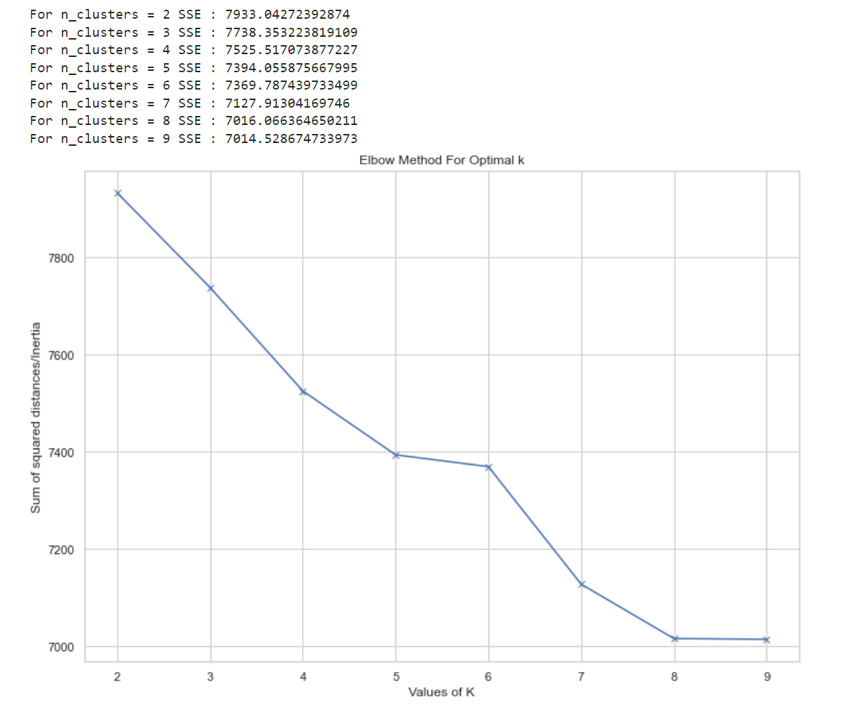
To classify the user into clusters, k-means algorithm will be used. An iteration with number of clusters from 2 to 9 is run and to decide the best number of clusters, it will be measured with SSE. This one method is chosen because of its simplicity. Once the number of clusters is decided, another iteration is run again until it no longer met specific threshold (sse > 7000). Once this process is done, the frequency of each word in each cluster is counted and visualized in a wordcloud since it is more readable than table.
matrix = X.values
sum_of_squared_distances = []
k = range(2,10)

for n_clusters in k:
    kmeans = KMeans(init='k-means++', n_clusters = n_clusters, n_init=30)
    kmeans.fit(matrix)
    clusters = kmeans.fit_predict(matrix)
    print("For n_clusters =", n_clusters, "SSE :", kmeans.inertia_)
    sum_of_squared_distances.append(kmeans.inertia_)
plt.plot(k, sum_of_squared_distances, 'bx-')
plt.xlabel('Values of K')
plt.ylabel('Sum of squared distances/Inertia')
plt.title('Elbow Method For Optimal k')
plt.show()
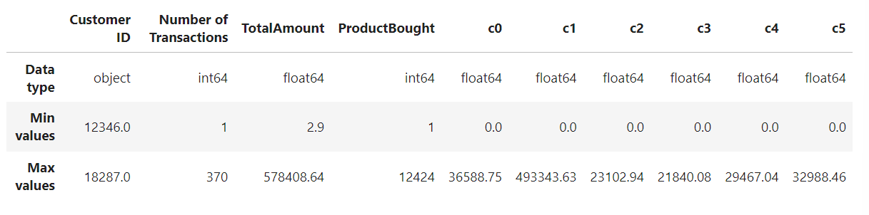
This code below measure the amount of money spent in each category. At first, new column that represents the seven category cluster is made. If the value of column Cluster match the number in cx with x = cluster, PaymentAmount from Price x (Quantity - QuantityCancelled) will be assigned to that new category column.
for i in range(7):
    col = 'c{}'.format(i)
    df_temp = df_clean[df_clean['Clusters'] == i]
    price_temp = df_temp['Price'] * (df_temp['Quantity'] - df_temp['QuantityCancelled'])
    price_temp = price_temp.apply(lambda x:x if x > 0 else 0)
    df_clean.loc[:, col] = price_temp
    df_clean[col].fillna(0, inplace = True)
df_clean
The codes below are used to group the data by its Customer ID and Invoice, and then sum the PaymentAmount as TotalAmount and count the PaymentAmount as ProductBought. Another iteration is also run to sum the amount of payment in each category per invoice and customer ID.
tmp = df_clean.groupby(by=['Customer ID','Invoice'], as_index=False)['Payment amount'].agg(['sum','count']).reset_index().rename(columns={'sum': 'TotalAmount', 'count': 'ProductBought'})
df_tmp = tmp.copy()

for i in range(df_clean['Clusters'].nunique()):
    col = 'c{}'.format(i)
    tmp = df_clean.groupby(by=['Customer ID', 'Invoice'], as_index=False)[col].sum()
    df_tmp.loc[:, col] = tmp[col]

df_tmp = df_tmp[df_tmp['TotalAmount'] > 0]
df_tmp
After df_tmp is obtained, it is grouped by Customer ID and the Invoice will be counted to get number of transaction for each Customer ID.
Here, cols define the feature that will be used in customer clustering.
Because the range of columns in this dataset is different, a scaler is used to standarized the data. Here, standard scaler is chosen to normalize the data within particular range. StandardScaler() [6] transforms the dataset such that the resulting distribution’s mean value is zero and the standard deviation is one.
After standarization of data is done, the dimensionality is reduced by using PCA because according to [1], the dimensionality reduction may allow the data to be more easily visualized.
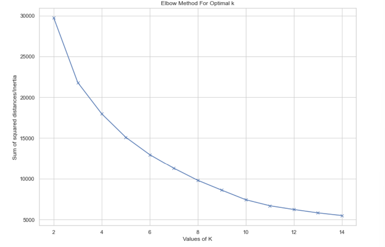
By measuring the clustering with SSE, n_clusters = 4 is choosen. After running the algorith on the scaled and dimentionally-reduced data, this is how the customer is clustered.
from itertools import cycle
import plotly as py

colors = cycle(py.colors.sequential.Electric)

layout = go.Layout(
    title= 'Clusters using Agglomerative Clustering',
    scene = dict(
            xaxis = dict(title  = 'Number of transactions'),
            yaxis = dict(title  = 'Total payment'),
            zaxis = dict(title  = 'Number of bought product')
        )
)
fig = go.Figure(layout=layout)
for s in df_usr['CustomerCluster'].unique():
    df = df_usr[df_usr['CustomerCluster'] == s]
    fig.add_trace(go.Scatter3d(x=df['Number of Transactions'], y = df['TotalAmount'], z = df['ProductBought'],
                               mode = 'markers',
                               name = s,
                               marker=dict(
                                   size= 6,
                                   opacity=0.65,
                               ),
                               marker_color = next(colors)))
fig.update_layout(autosize=False,
    width=750,
    height=750,
    margin=dict(
        l=50,
        r=50,
        b=100,
        t=100,
        pad=4), legend = dict(orientation="h", x = 1, y = 0.7, title = 'Clusters'))
fig.update_traces(legendgroup='CustCluster', selector=dict(type='scatter3d'))
fig.show()
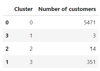
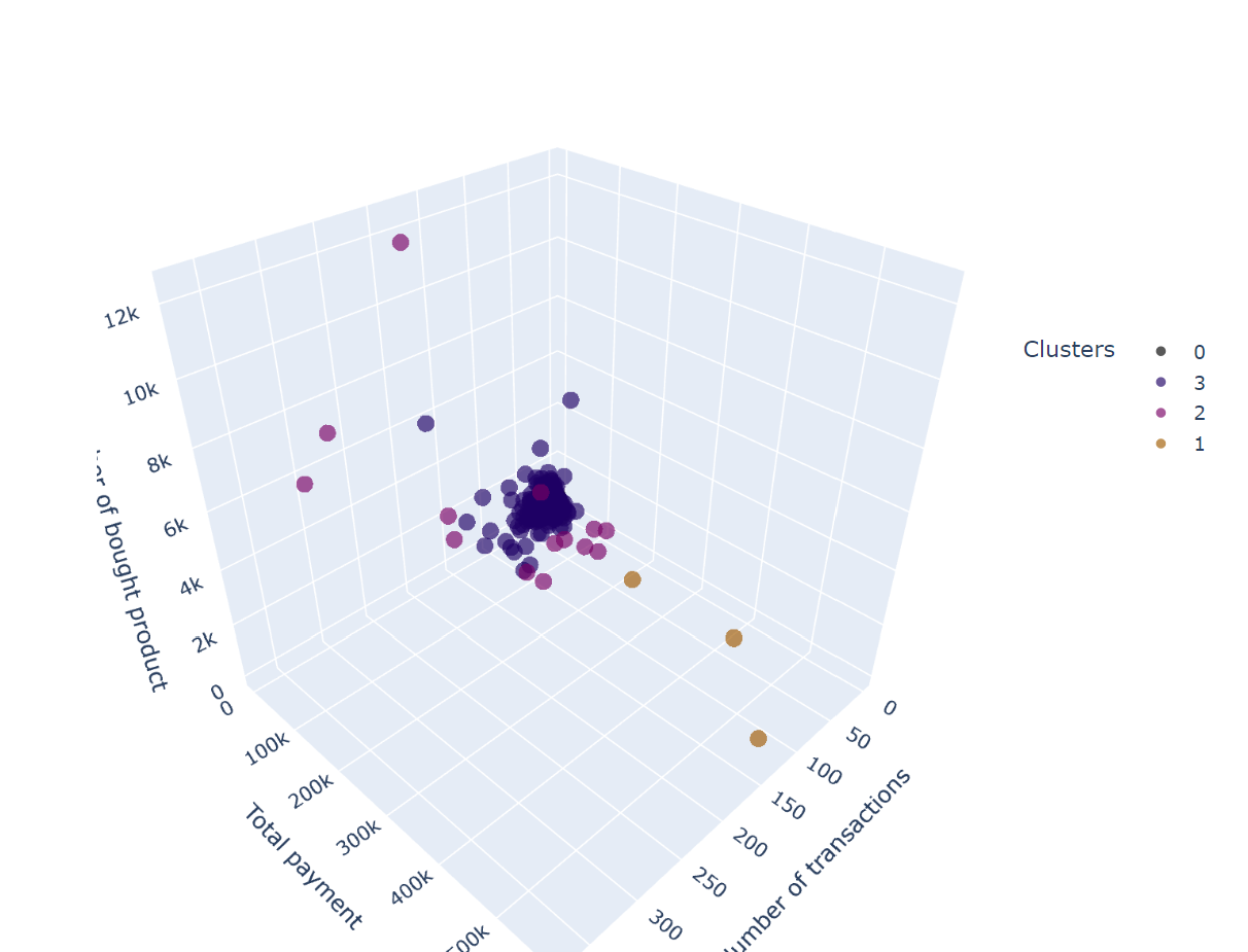
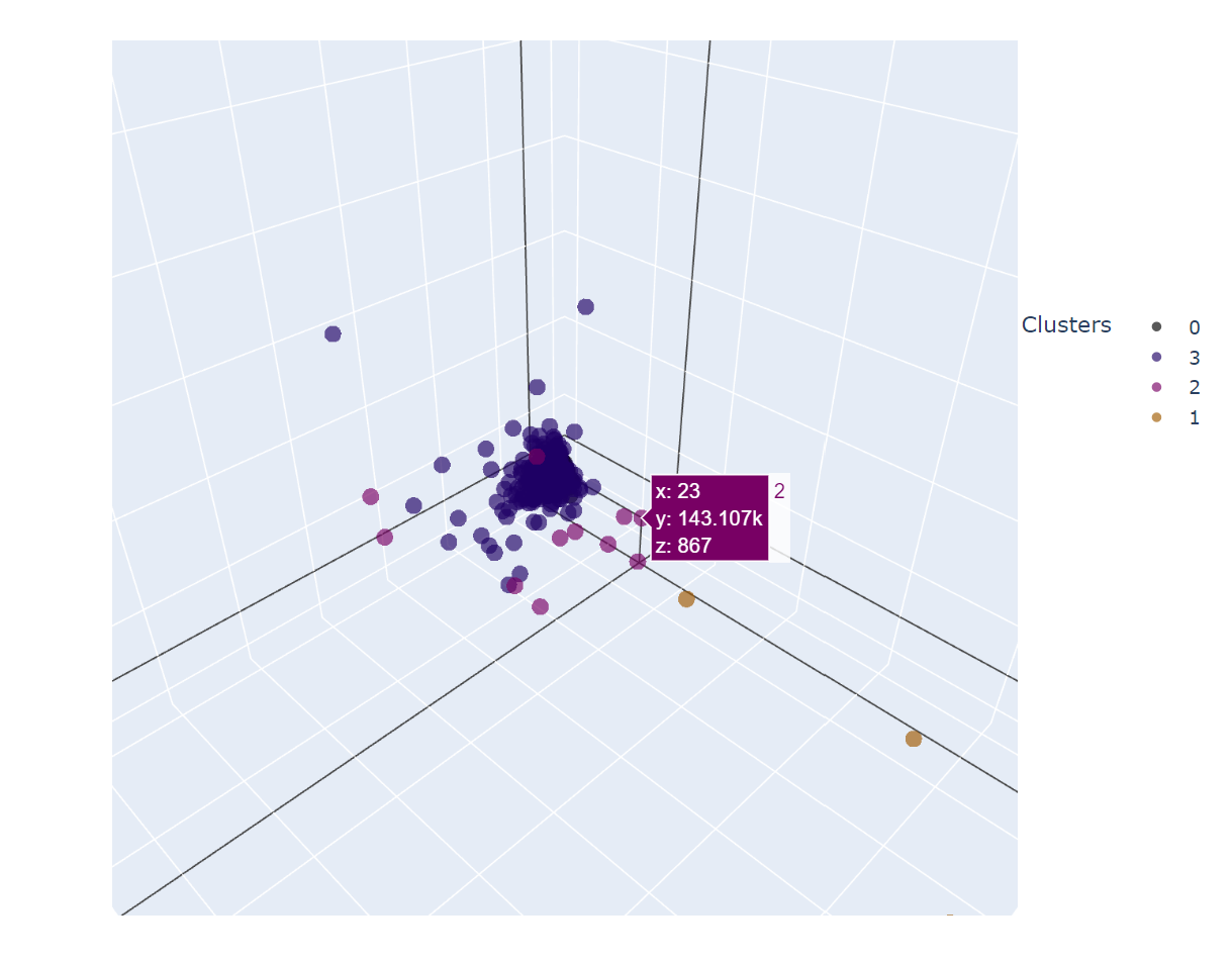
From the visualization above, some insight of customer’s buying pattern that is obtained are:
- Cluster 0: low number of transaction, total payment, and number of bought product
- Cluster 3: higher number of transaction, total payment, and number of bought product compared to cluster 0
- CLuster 1: customer with frequent buying
- Cluster 2: non-frequent buying but total payment in each transaction is high